2010 US Census data
The 2010 Census collected a variety of demographic information for all the more than 300 million people in the USA. Here we’ll focus on the subset of the data selected by the Cooper Center, who produced a map of the population density and the racial makeup of the USA. Each dot in this map corresponds to a specific person counted in the census, located approximately at their residence. (To protect privacy, the precise locations have been randomized at the census block level, so that the racial category can only be determined to within a rough geographic precision.) The Cooper Center website delivers pre-rendered tiles, which are fast to view but limited to the specific plotting choices they made. Here we will show how to run novel analyses focusing on whatever aspects of the data that you select yourself, rendered dynamically as requested using the datashader library.
Load data and set up
First, let’s load this data into a Dask dataframe. Dask is similar to Pandas, but with extra support for distributed or out-of-core (larger than memory) operation. If you have at least 16GB of RAM, you should be able to run this notebook-as is, using fast in-core operations. If you have less memory, you’ll need to use the slower out-of-core operations by commenting out the .persist() call.
import datashader as ds
import datashader.transfer_functions as tf
import dask.dataframe as dd
import numpy as np
import pandas as pd
%%time
df = dd.io.parquet.read_parquet('data/census.snappy.parq')
df = df.persist()
CPU times: user 29.3 s, sys: 4.51 s, total: 33.8 s
Wall time: 18.3 s
df.head()
| easting | northing | race | |
|---|---|---|---|
| 0 | -13700737.0 | 6275190.0 | w |
| 1 | -13700711.0 | 6275195.0 | w |
| 2 | -13702081.0 | 6274898.5 | w |
| 3 | -13701948.0 | 6274931.0 | w |
| 4 | -13701793.0 | 6275088.5 | w |
There are 306675004 rows in this dataframe (one per person counted in the census), each with a location in Web Mercator format and a race encoded as a single character (where ‘w’ is white, ‘b’ is black, ‘a’ is Asian, ‘h’ is Hispanic, and ‘o’ is other (typically Native American)). (Try len(df) to see the size, if you want to check, though that forces the dataset to be loaded so it’s skipped here.)
Let’s define some geographic ranges to look at later, and also a default plot size. Feel free to increase plot_width to 2000 or more if you have a very large monitor or want to save big files to disk, which shouldn’t greatly affect the processing time or memory requirements.
USA           = ((-124.72,  -66.95), (23.55, 50.06))
LakeMichigan  = (( -91.68,  -83.97), (40.75, 44.08))
Chicago       = (( -88.29,  -87.30), (41.57, 42.00))
Chinatown     = (( -87.67,  -87.63), (41.84, 41.86))
NewYorkCity   = (( -74.39,  -73.44), (40.51, 40.91))
LosAngeles    = ((-118.53, -117.81), (33.63, 33.96))
Houston       = (( -96.05,  -94.68), (29.45, 30.11))
Austin        = (( -97.91,  -97.52), (30.17, 30.37))
NewOrleans    = (( -90.37,  -89.89), (29.82, 30.05))
Atlanta       = (( -84.88,  -84.04), (33.45, 33.84))

from datashader.utils import lnglat_to_meters as webm
x_range,y_range = [list(r) for r in webm(*USA)]

plot_width  = int(900)
plot_height = int(plot_width*7.0/12)
Let’s also choose a background color for our results. A black background makes bright colors more vivid, and works well when later adding relatively dark satellite image backgrounds, but white backgrounds (background=None) are good for examining the weakest patterns, and work well when overlaying on maps that use light colors. Try it both ways and decide for yourself!
background = "black"
We’ll also need some utility functions and colormaps, and to make the page as big as possible:
from functools import partial
from datashader.utils import export_image
from datashader.colors import colormap_select, Greys9
from colorcet import fire
from IPython.core.display import HTML, display

export = partial(export_image, background = background, export_path="export")
cm = partial(colormap_select, reverse=(background!="black"))

display(HTML("<style>.container { width:100% !important; }</style>"))
Population density
For our first examples, let’s ignore the race data for now, focusing on population density alone (as for the nyc_taxi.ipynb example). We’ll first aggregate all the points from the continental USA into a grid containing the population density per pixel:
%%time
cvs = ds.Canvas(plot_width, plot_height, *webm(*USA))
agg = cvs.points(df, 'easting', 'northing')
CPU times: user 1.79 s, sys: 14.3 ms, total: 1.8 s
Wall time: 691 ms
Computing this aggregate grid will take some CPU power (5 seconds on a MacBook Pro), because datashader has to iterate through the entire dataset, with hundreds of millions of points. Once the agg array has been computed, subsequent processing will now be nearly instantaneous, because there are far fewer pixels on a screen than points in the original database.
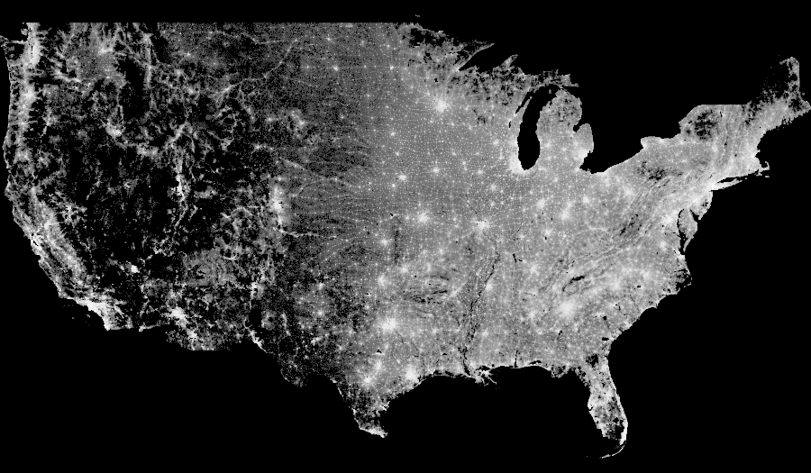
If we now plot the aggregate grid linearly, we can clearly see…
The above plot reveals at least that data has been measured only within the political boundaries of the continental United States, and also that many areas in the West are so poorly populated that many pixels contained not even a single person. (In datashader images, the background color is shown for pixels that have no data at all, using the alpha channel of a PNG image, while the colormap range is shown for pixels that do have data.) Some additional population centers are now visible, at least on some monitors. But mainly what the above plot indicates is that population in the USA is extremely non-uniformly distributed, with hotspots in a few regions, and nearly all other pixels having much, much lower (but nonzero) values. Again, that’s not much information to be getting out out of 300 million datapoints!
The problem is that of the available intensity scale in this gray colormap, nearly all pixels are colored the same low-end gray value, with only a few urban areas using any other colors. Thus this version of the map conveys very little information as well. Because the data are clearly distributed so non-uniformly, let’s instead try a nonlinear mapping from population counts into the colormap. A logarithmic mapping is often a good choice:
export(tf.shade(agg, cmap = cm(Greys9,0.2), how='log'),"census_gray_log")